Walking Fingerprinting
Using Functional Data Analysis
4/15/25
Follow along

Introduction
- 4th year PhD candidate in biostatistics at Johns Hopkins
- Advisor: Ciprian Cranineanu
- Wearable and Implantable Technology (WIT) research group
- Interests: accelerometry, functional data, walking
Problem description
What do I mean “walking fingerprinting”?
Problem description
What do I mean “walking fingerprinting”?
Applications


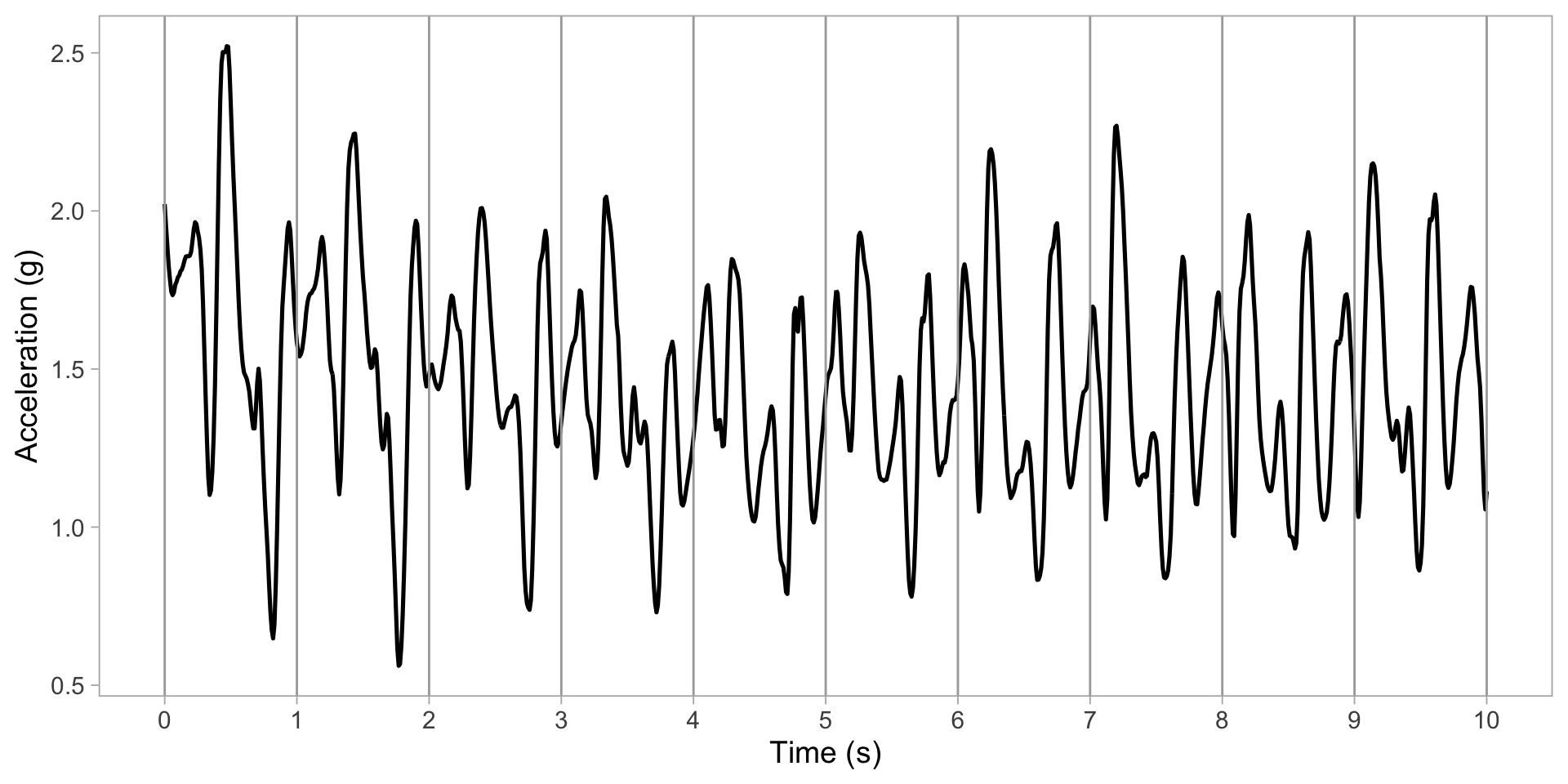
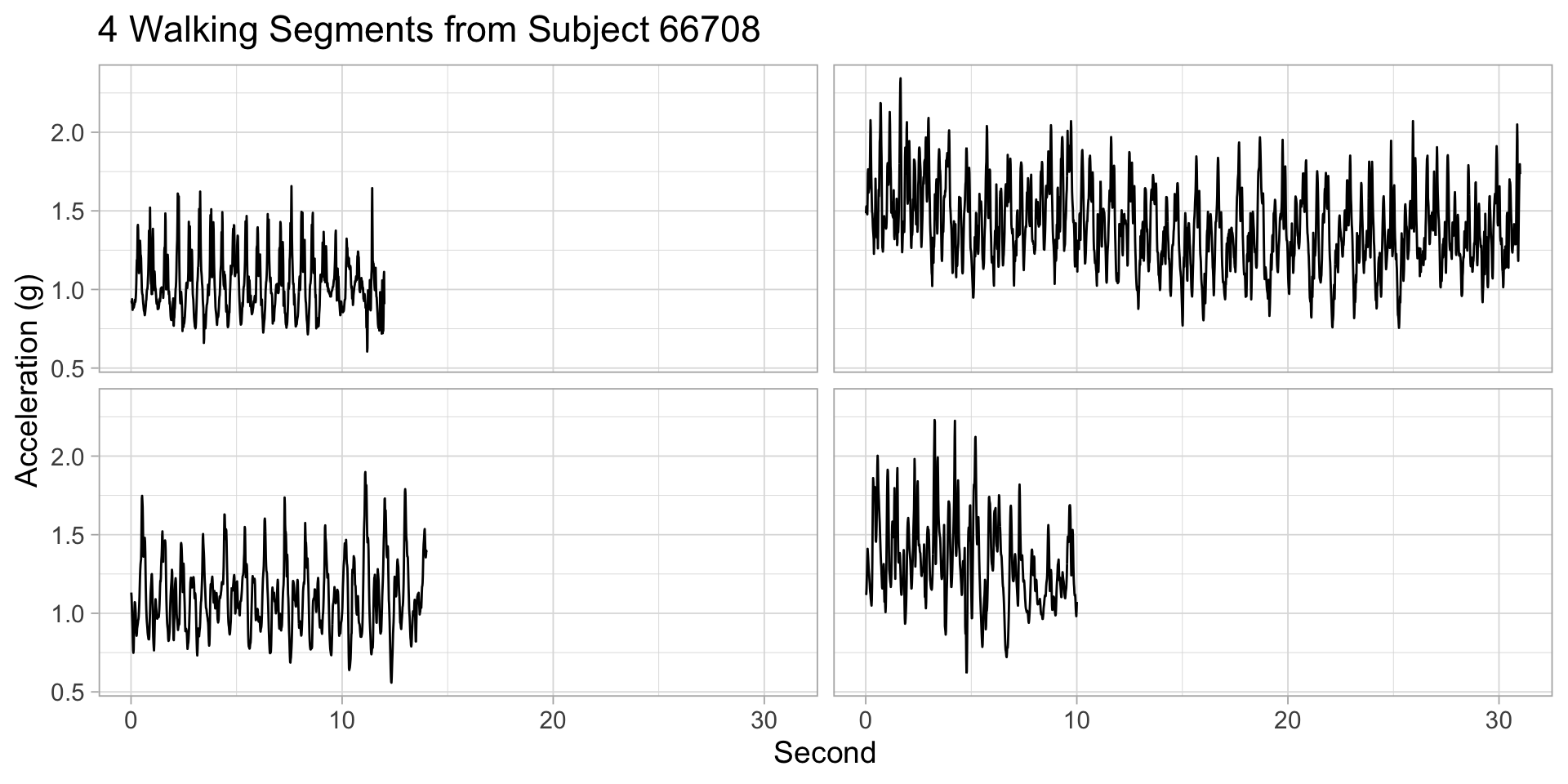
Backing up: accelerometry
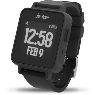
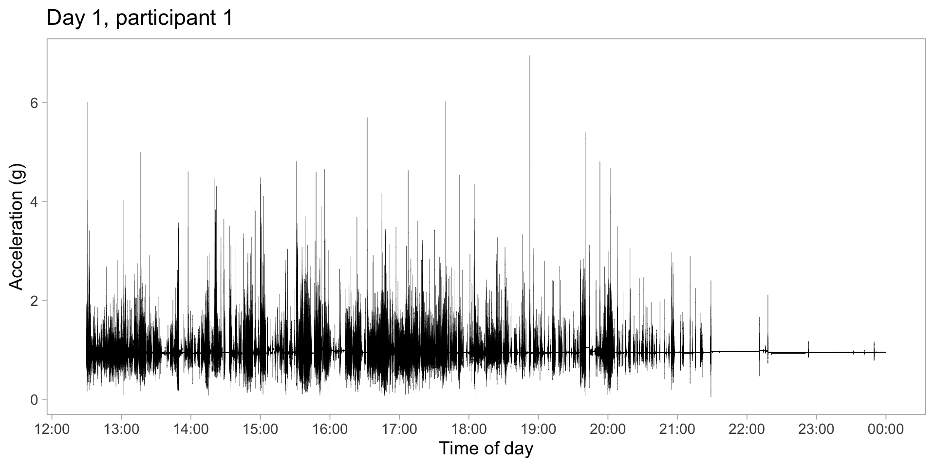
Accelerometry: collected from a wearable device
Between 15 and 100 observations per second in 3 dimensions
\(g\) units = 9.81 \(m/s^2\)
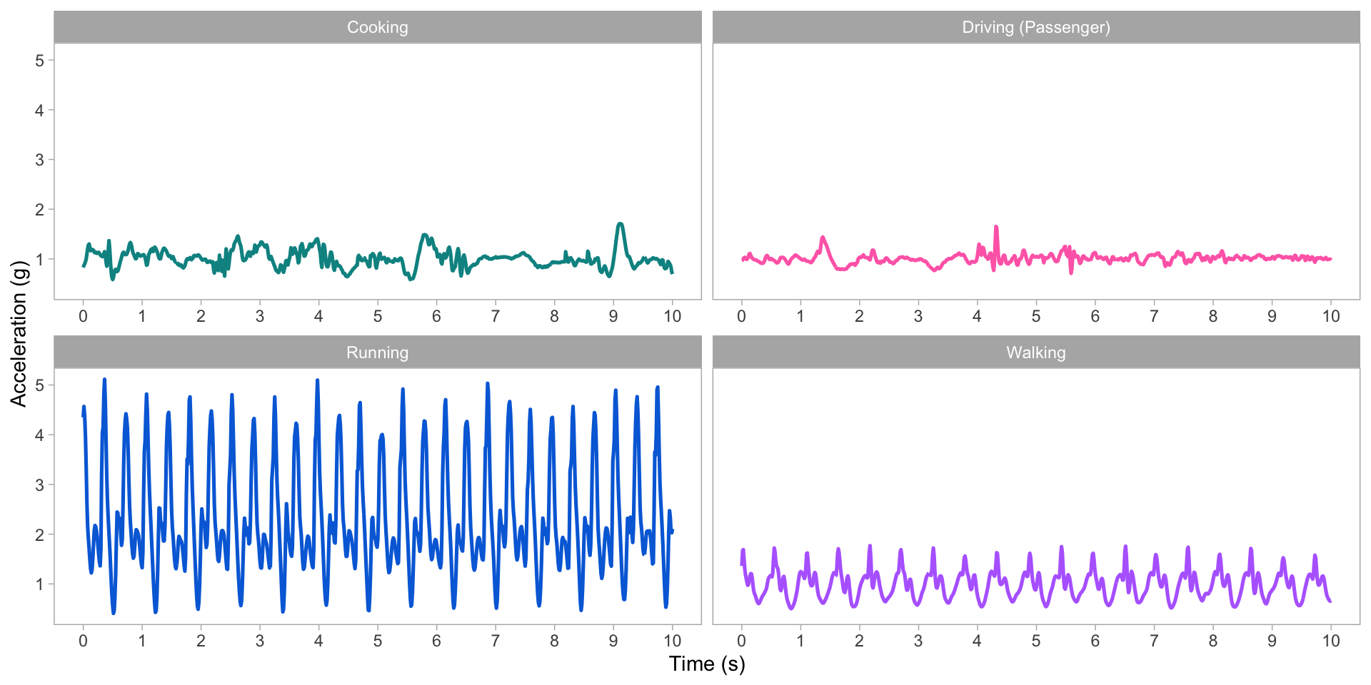
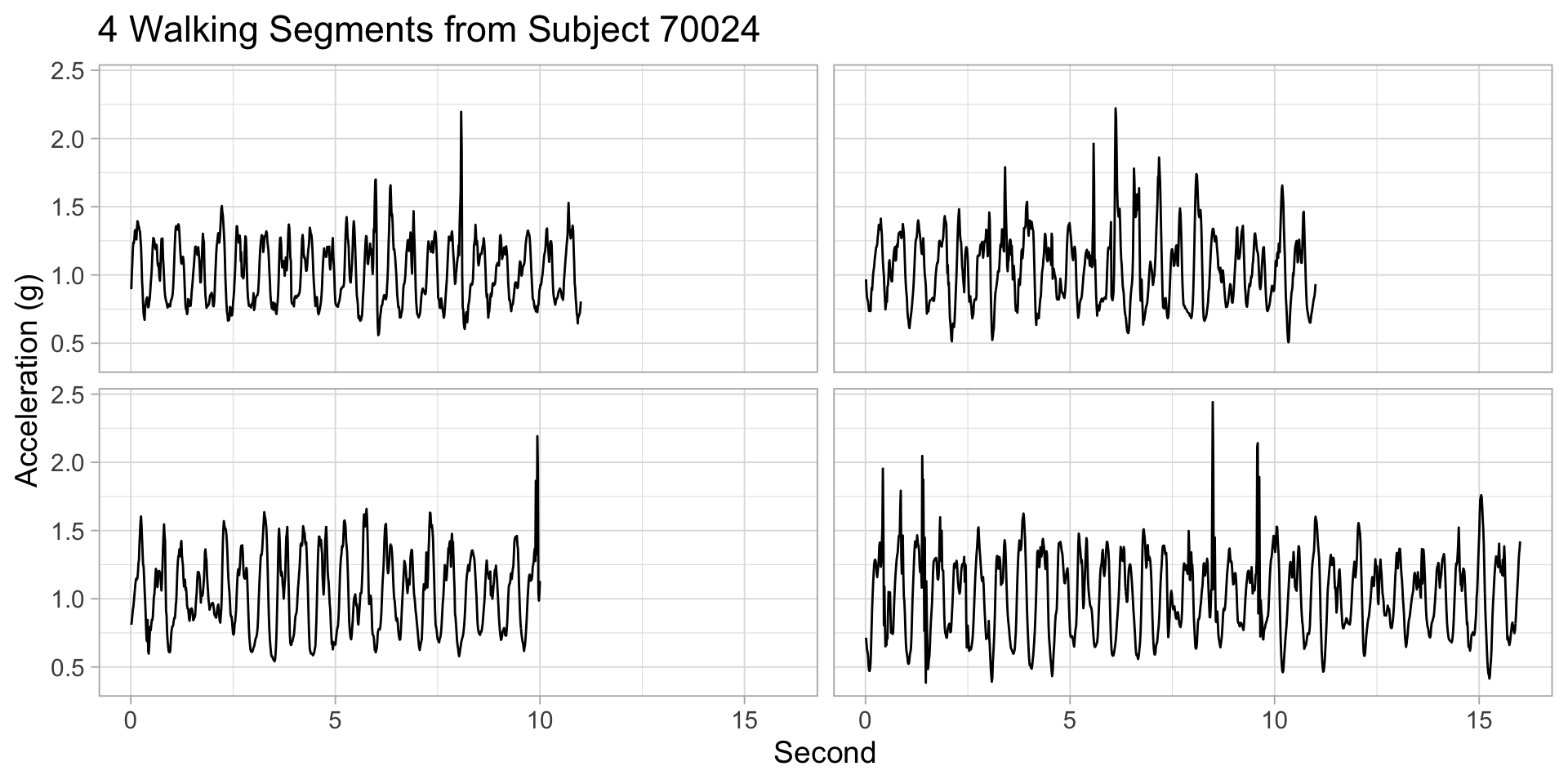
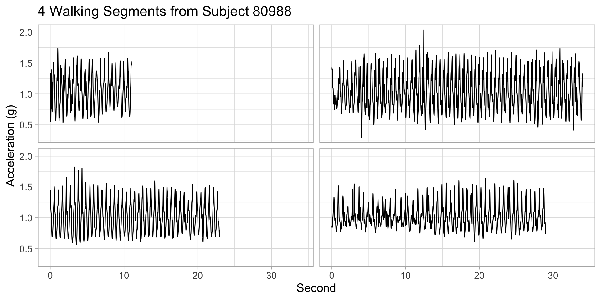
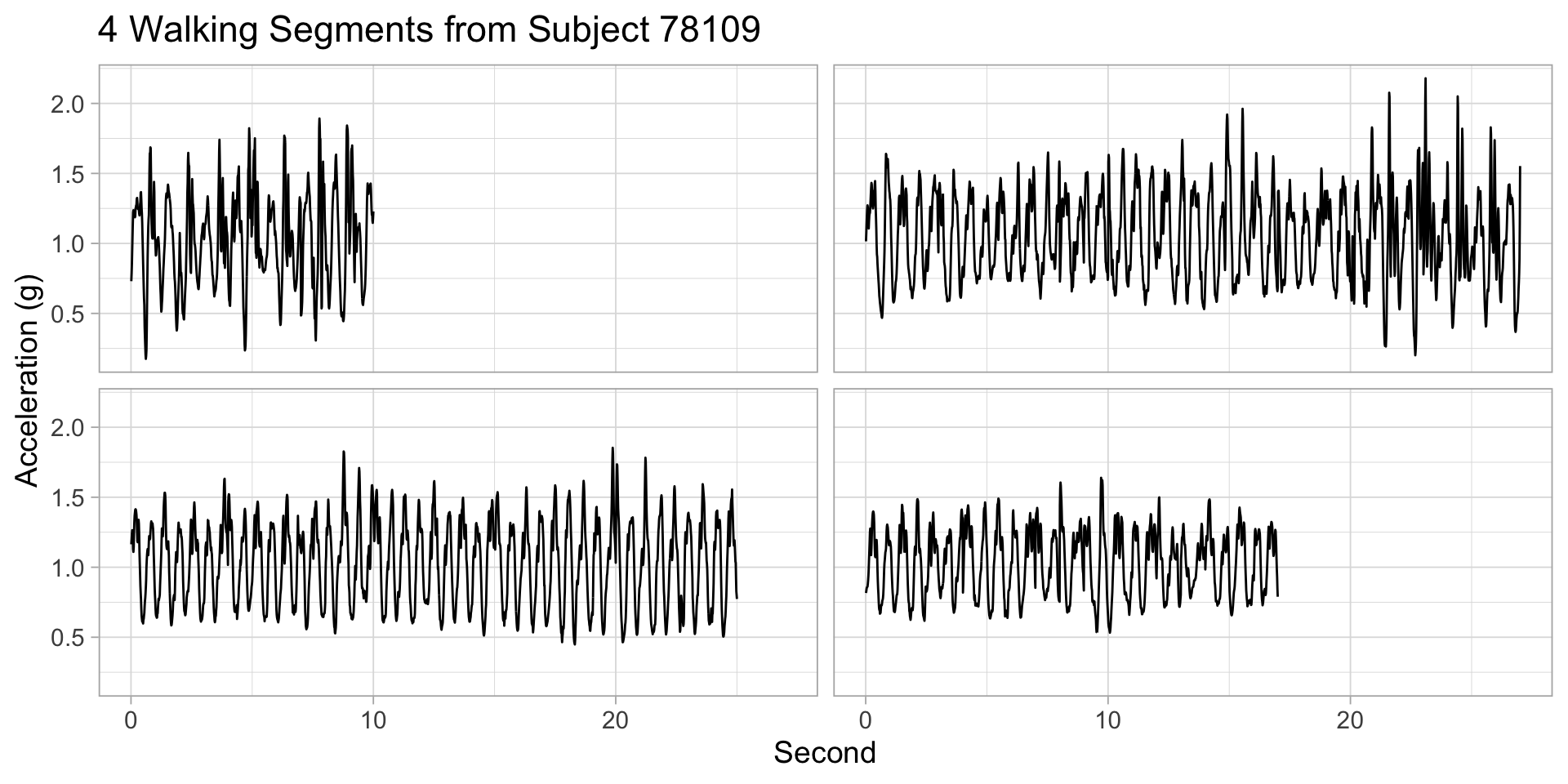
Accelerometry data
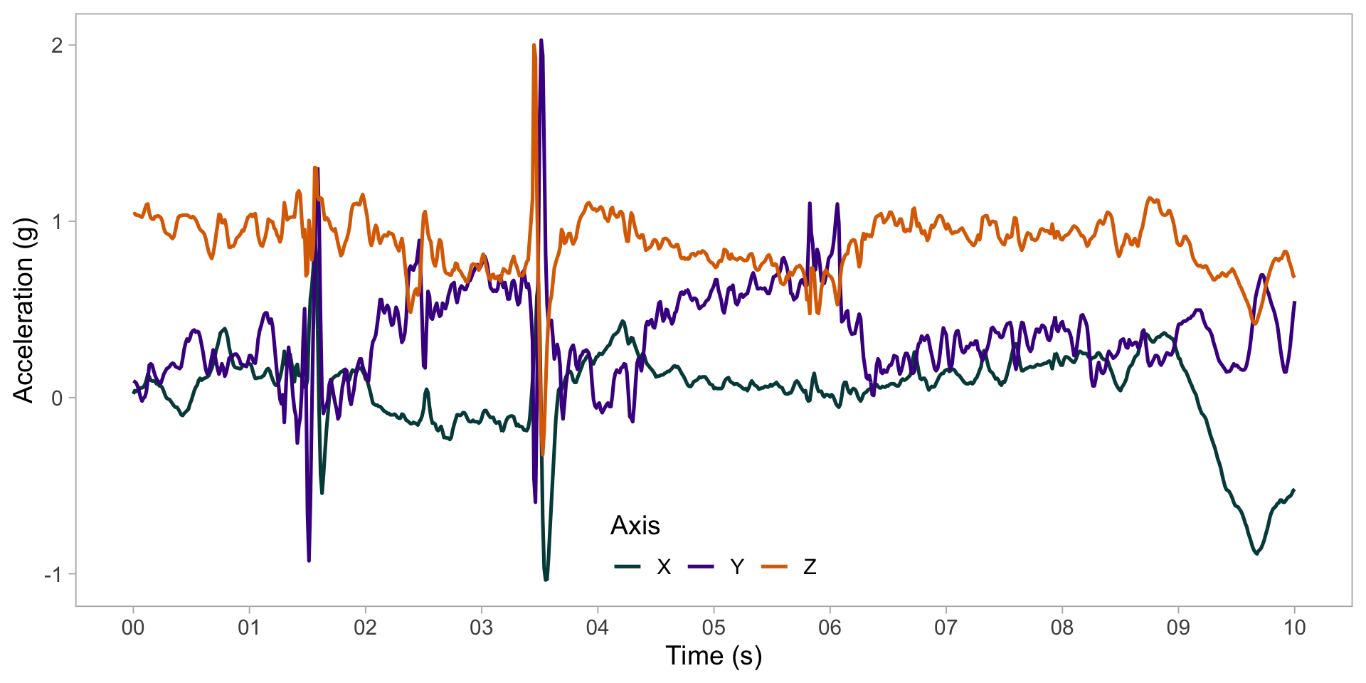
Accelerometry data
Accelerometry data
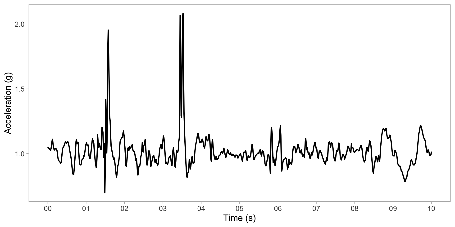
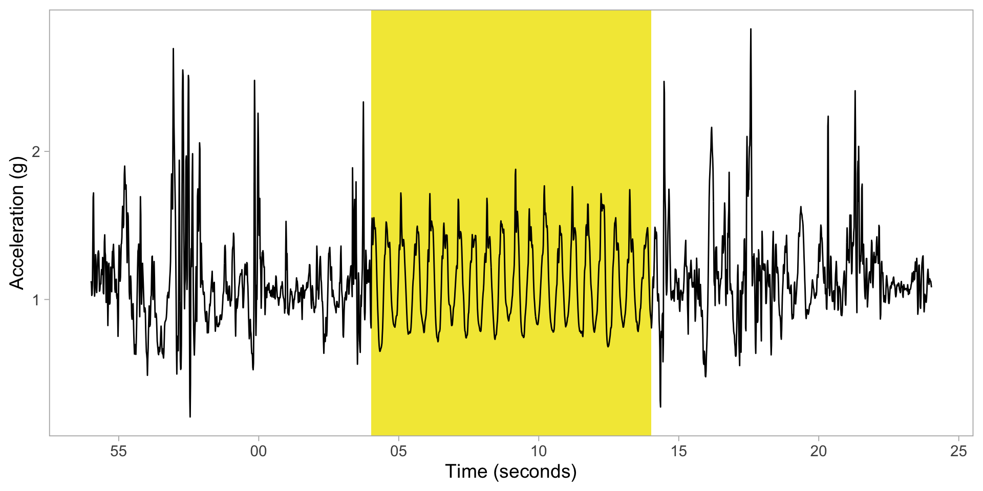
Segment data into 1-s chunks
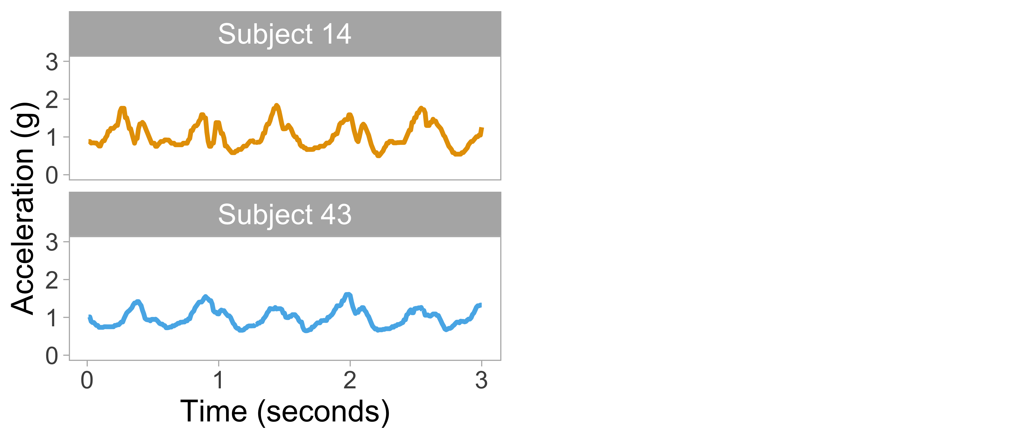
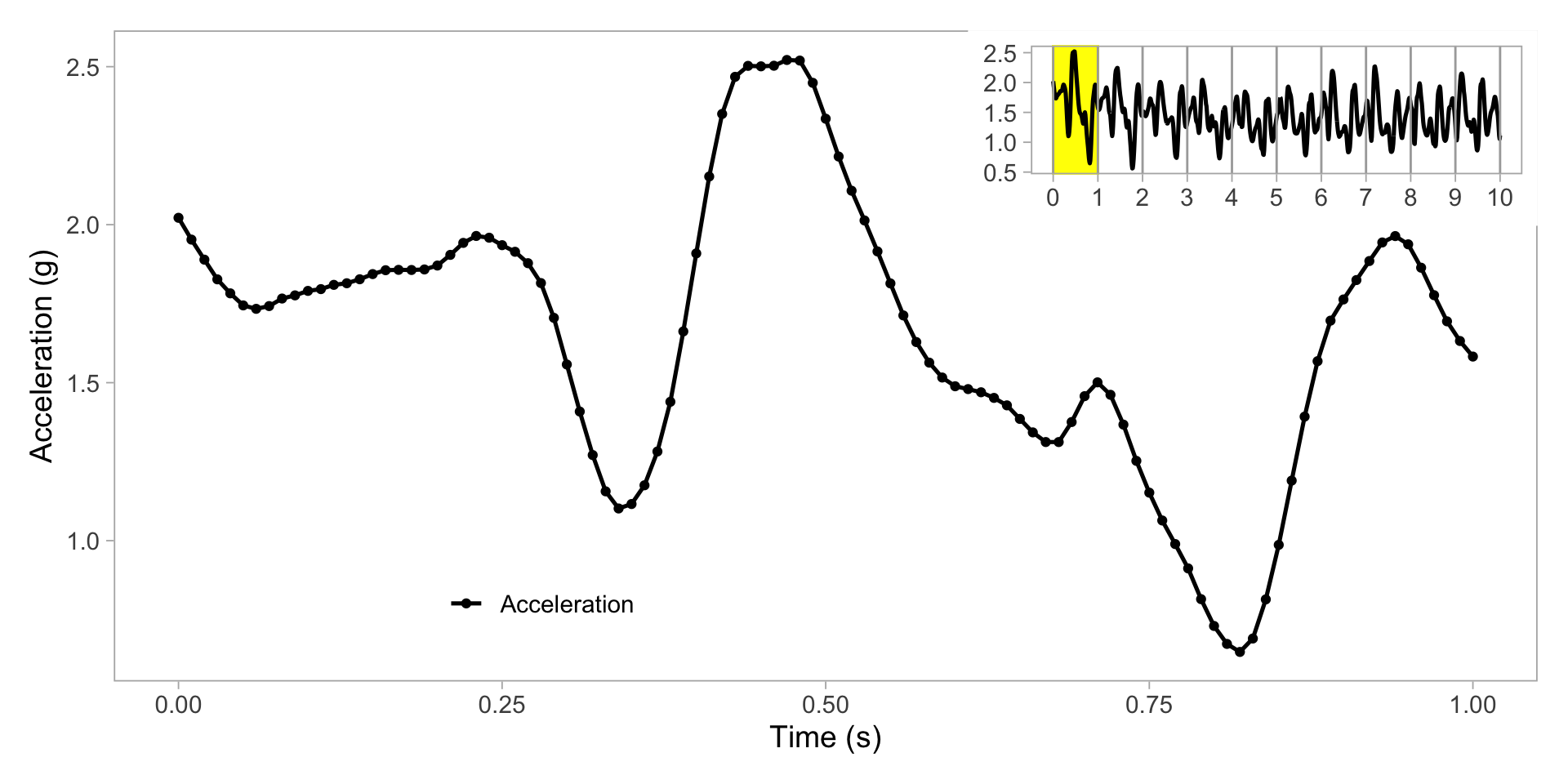
Zoom in on one second
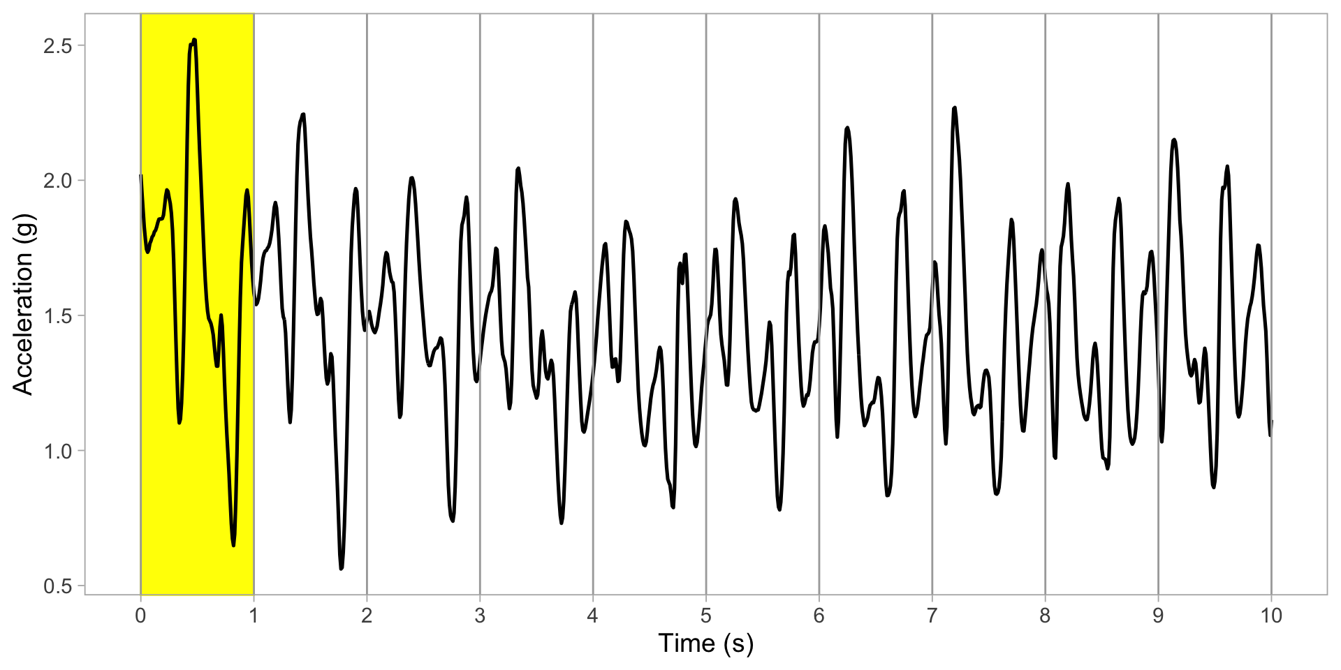
Zoom in on one second
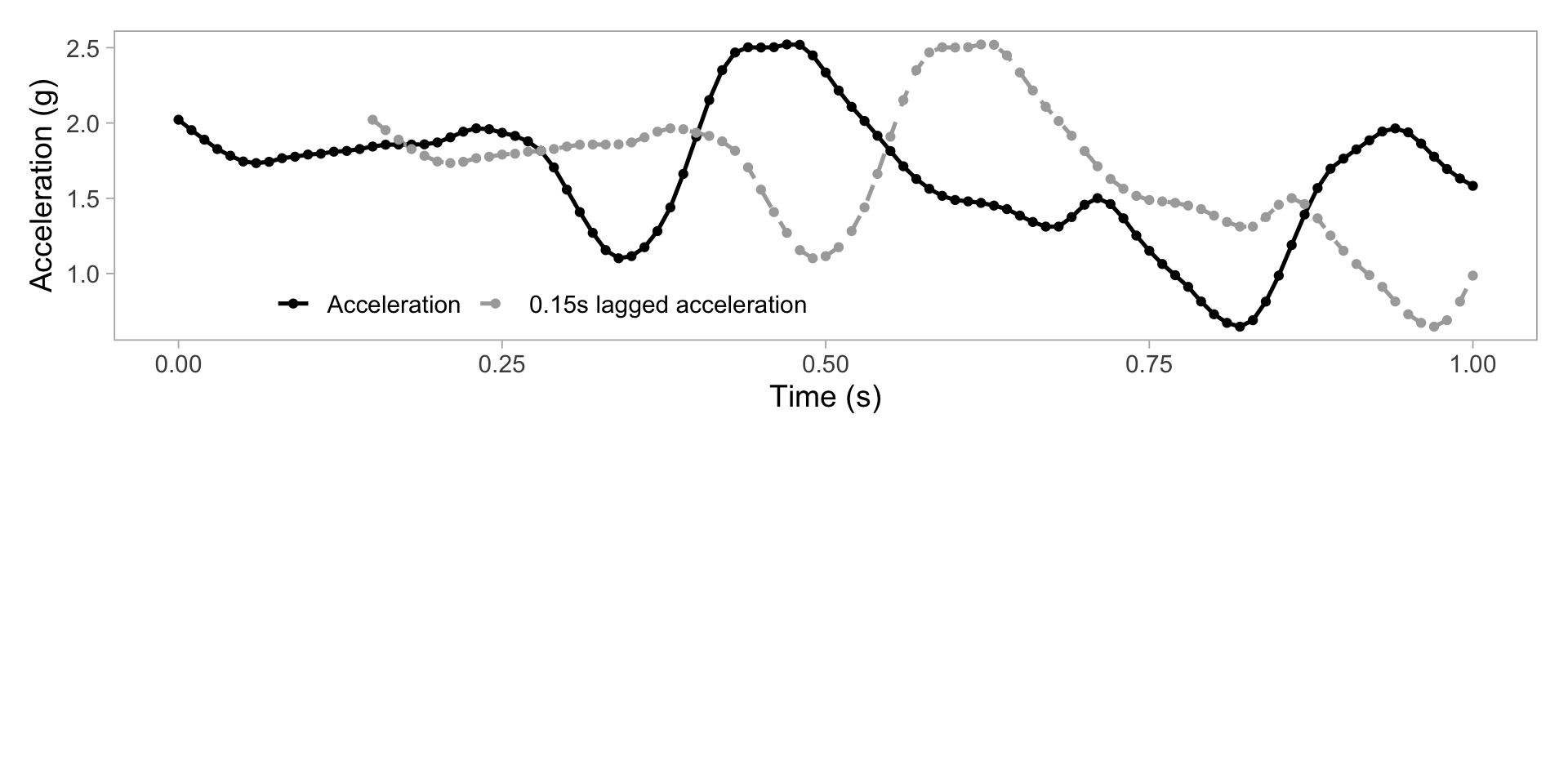
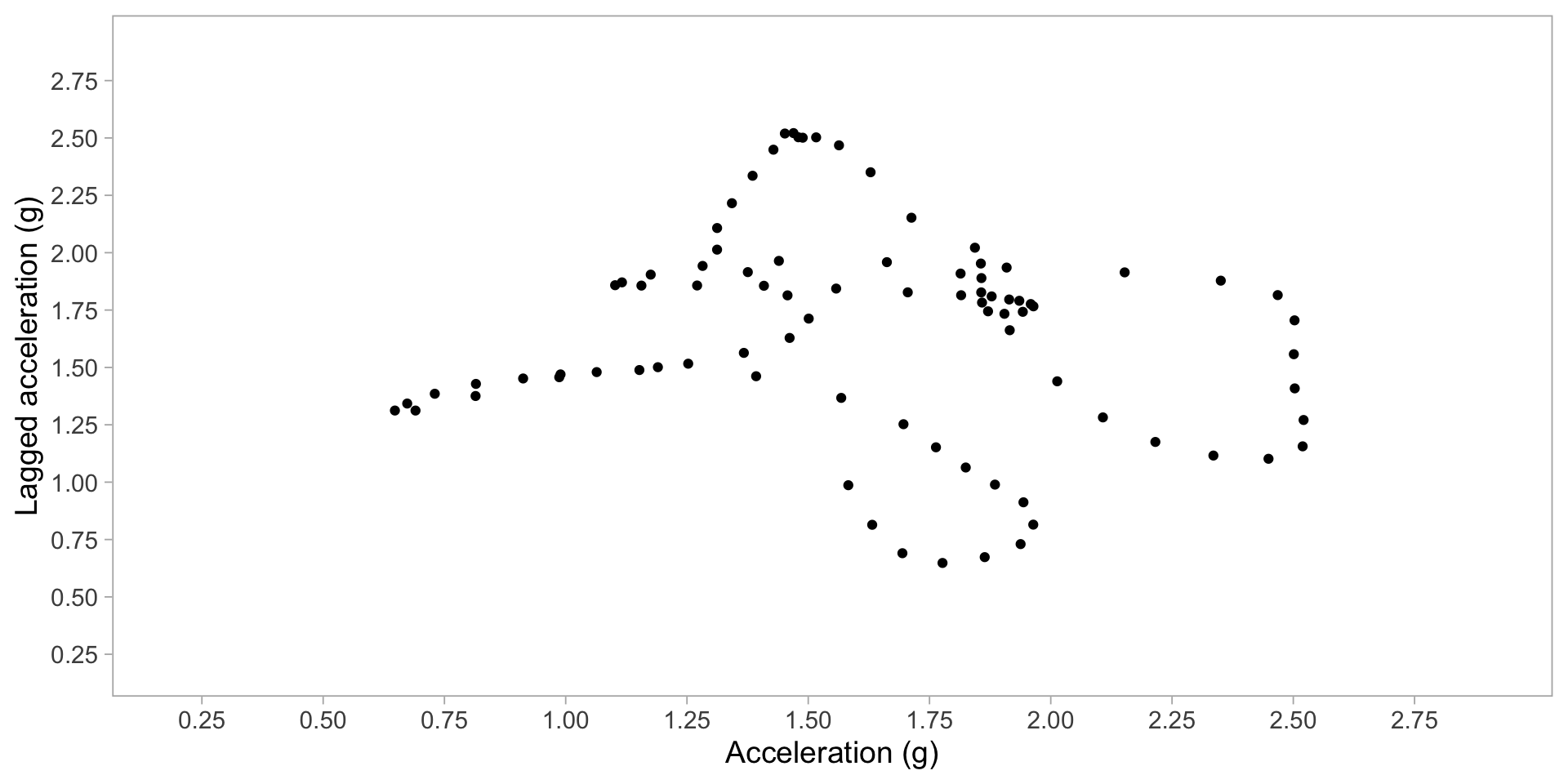
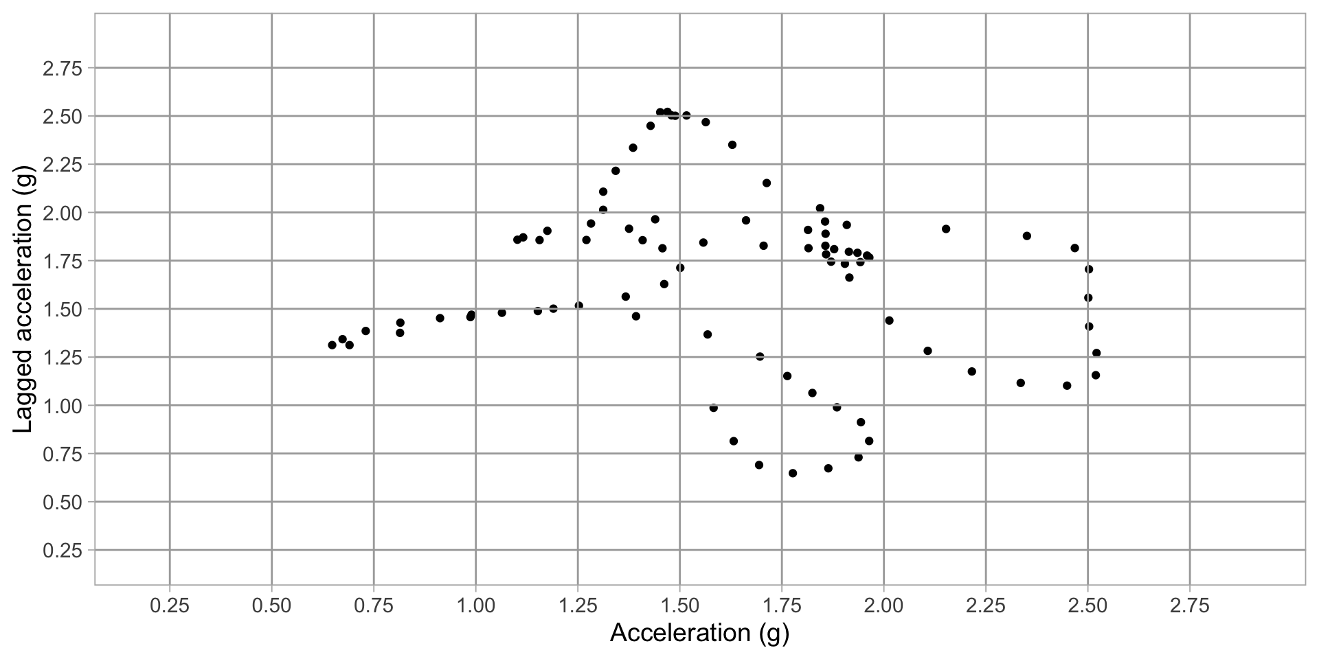
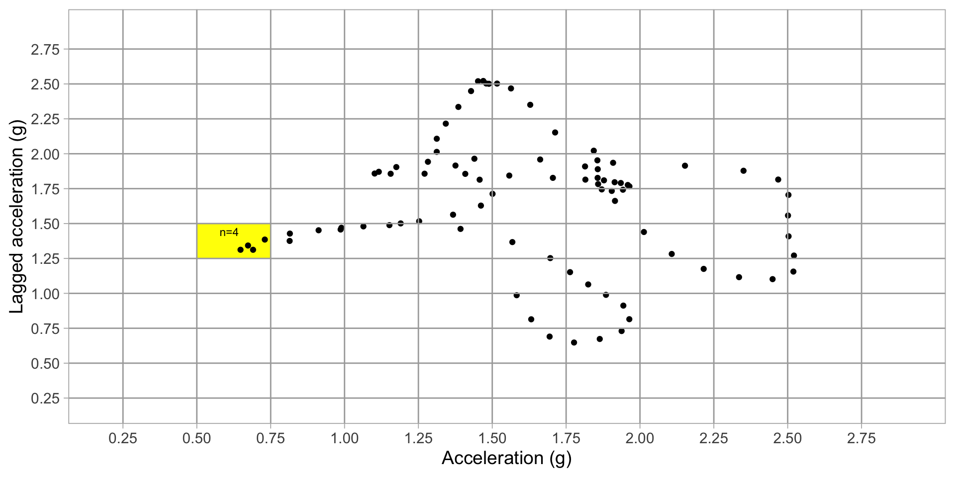
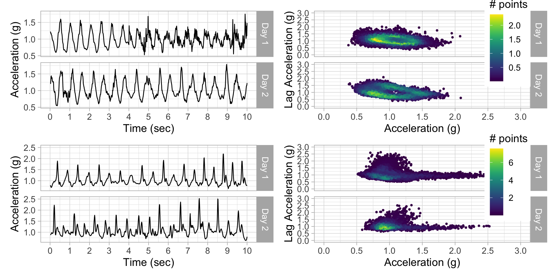
Plot acceleration, lag acceleration
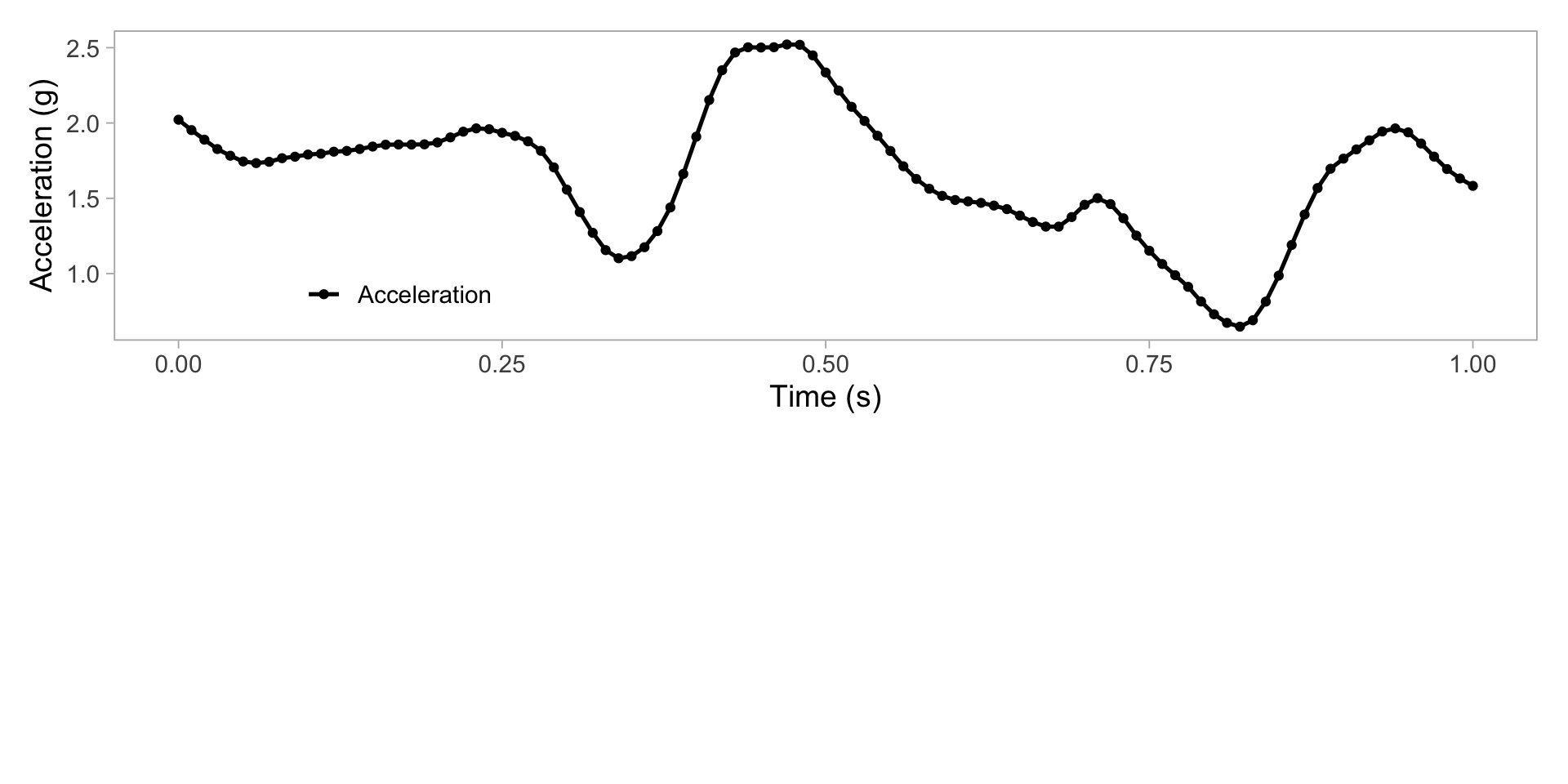
Plot acceleration, lag acceleration
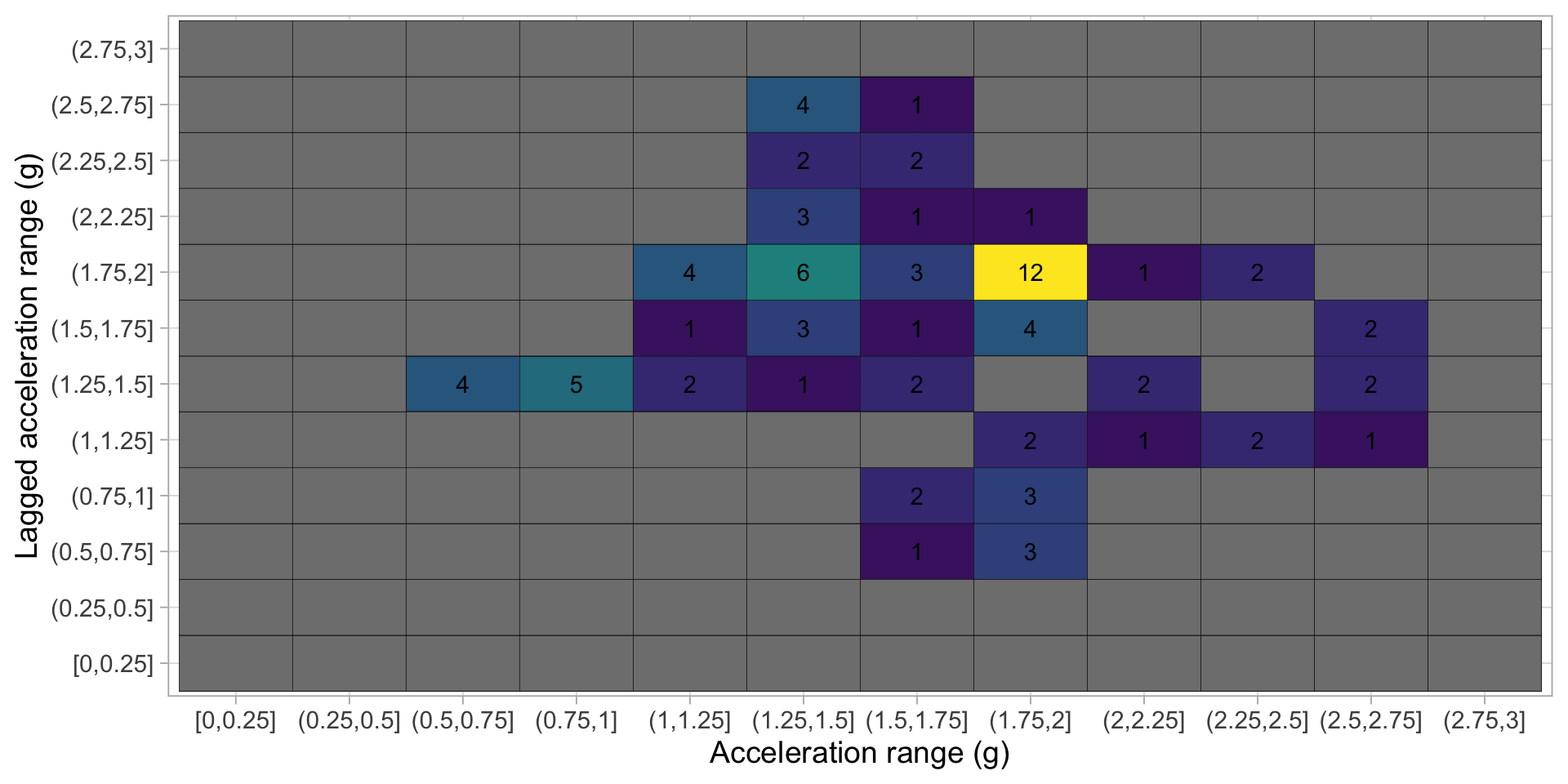
Transform to 2D grid
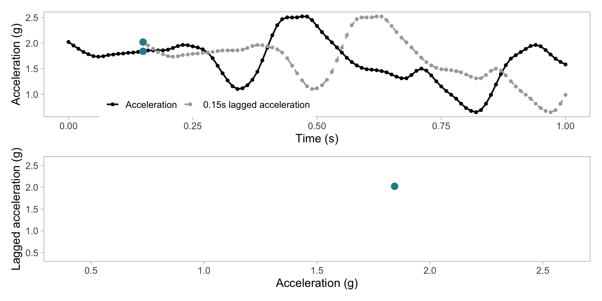
Transform acceration to 2D grid
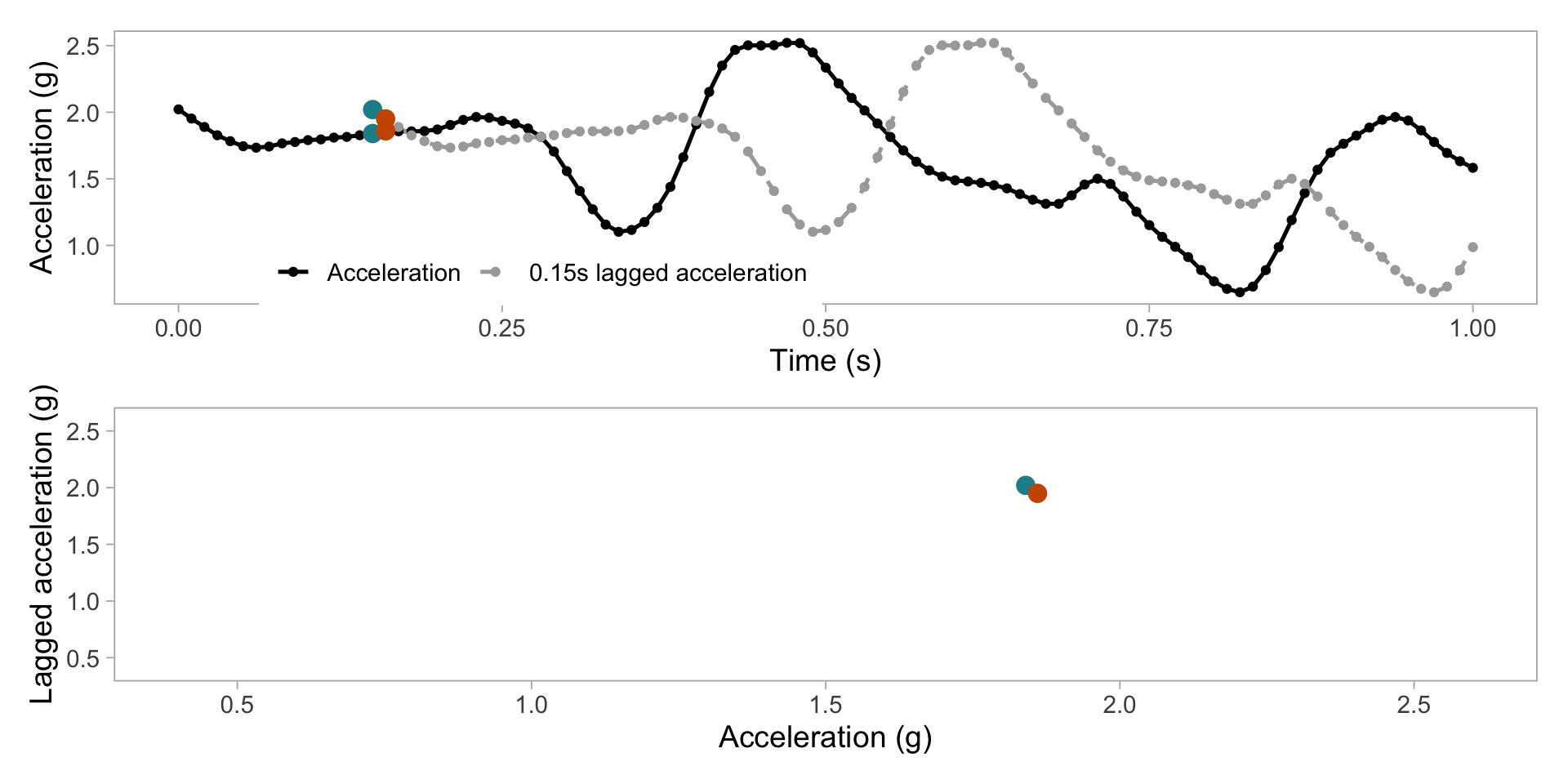
Transform acceration to 2D grid
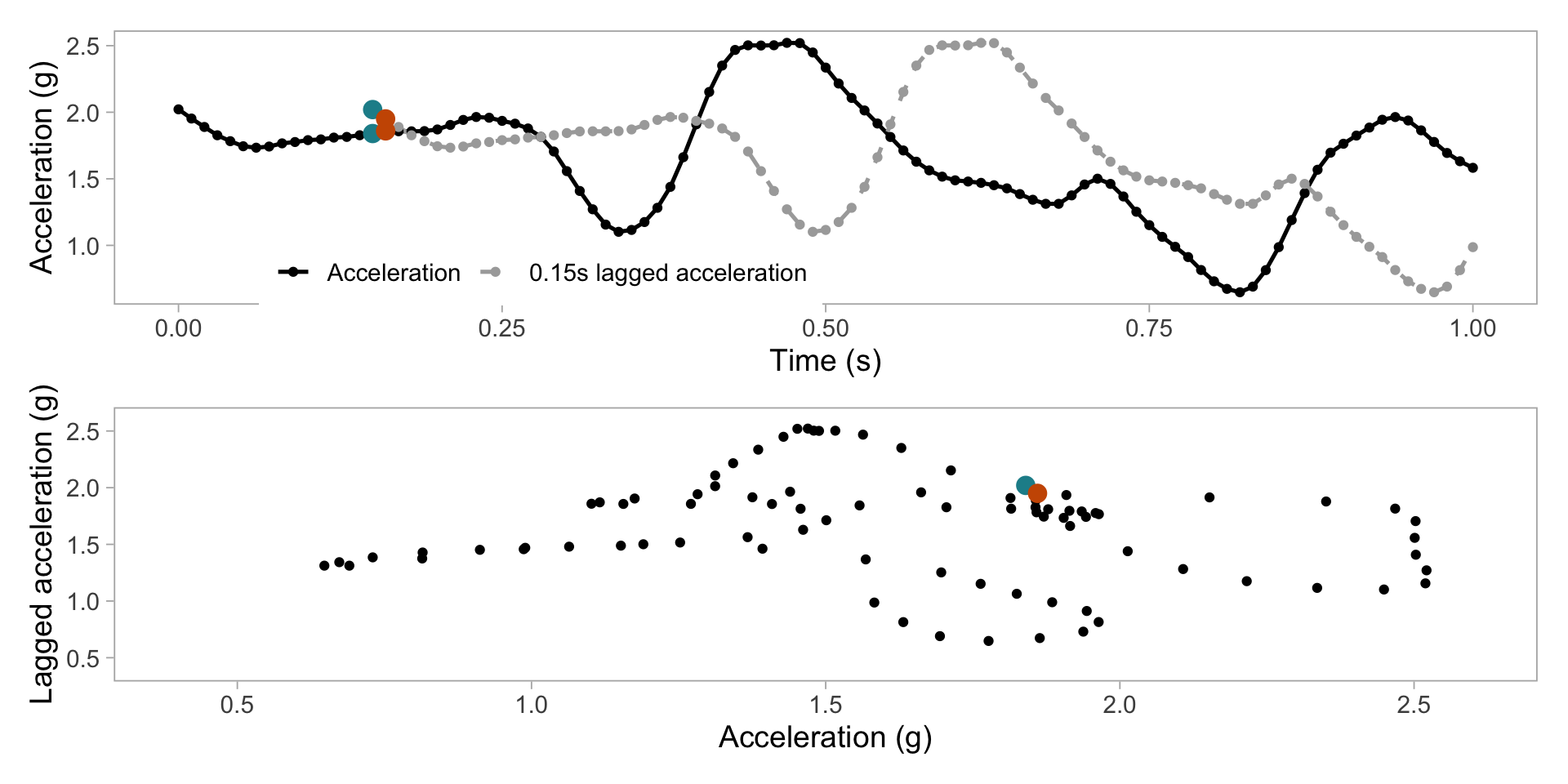
Transform to 2D grid
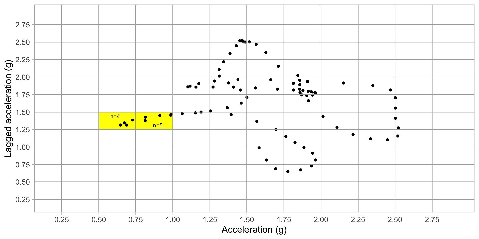
Derive predictors from grid
Derive predictors from grid
Derive predictors from grid
Derive predictors from grid
Derive predictors from the grid
Derive predictors from the grid
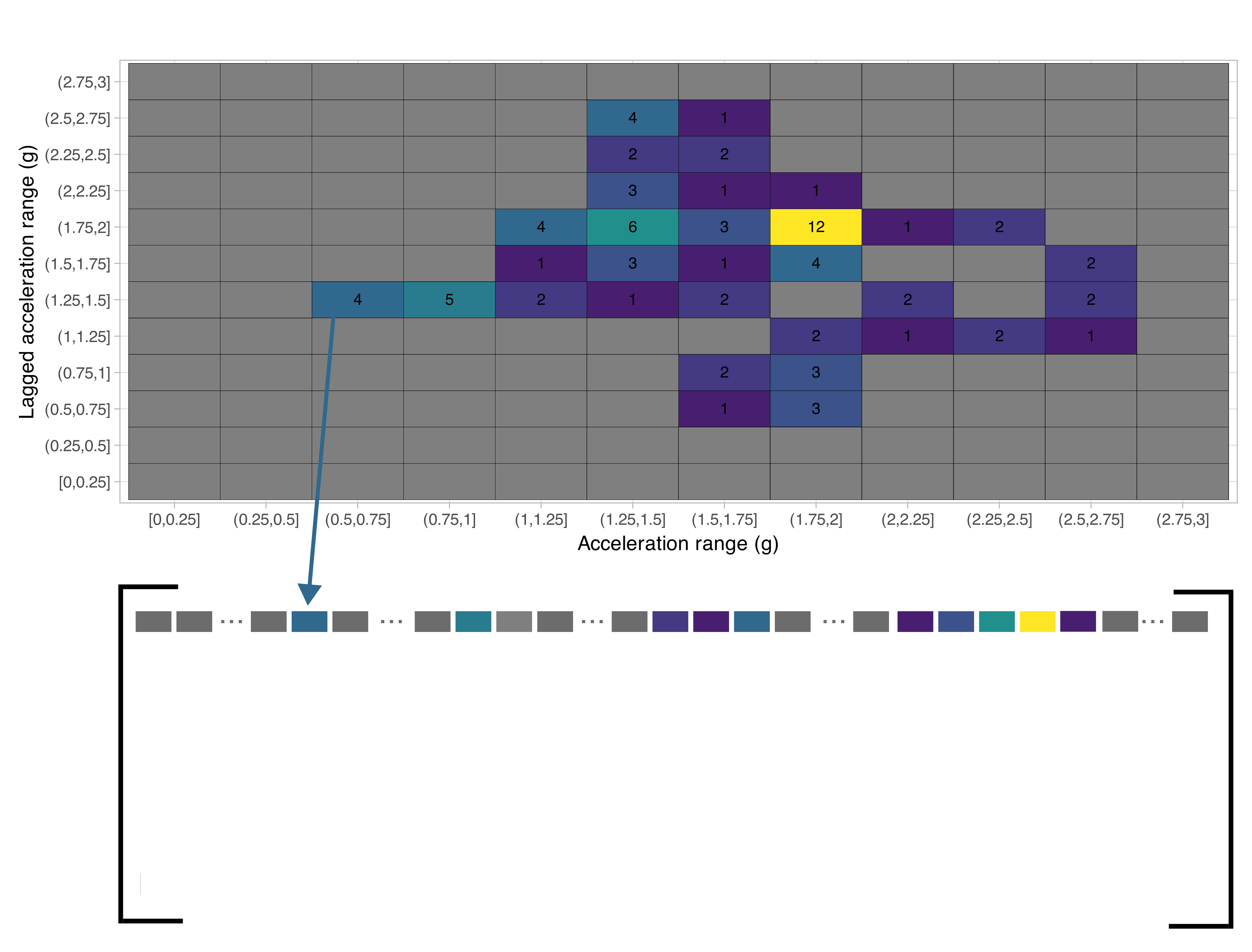
Derive predictors: repeat for all seconds
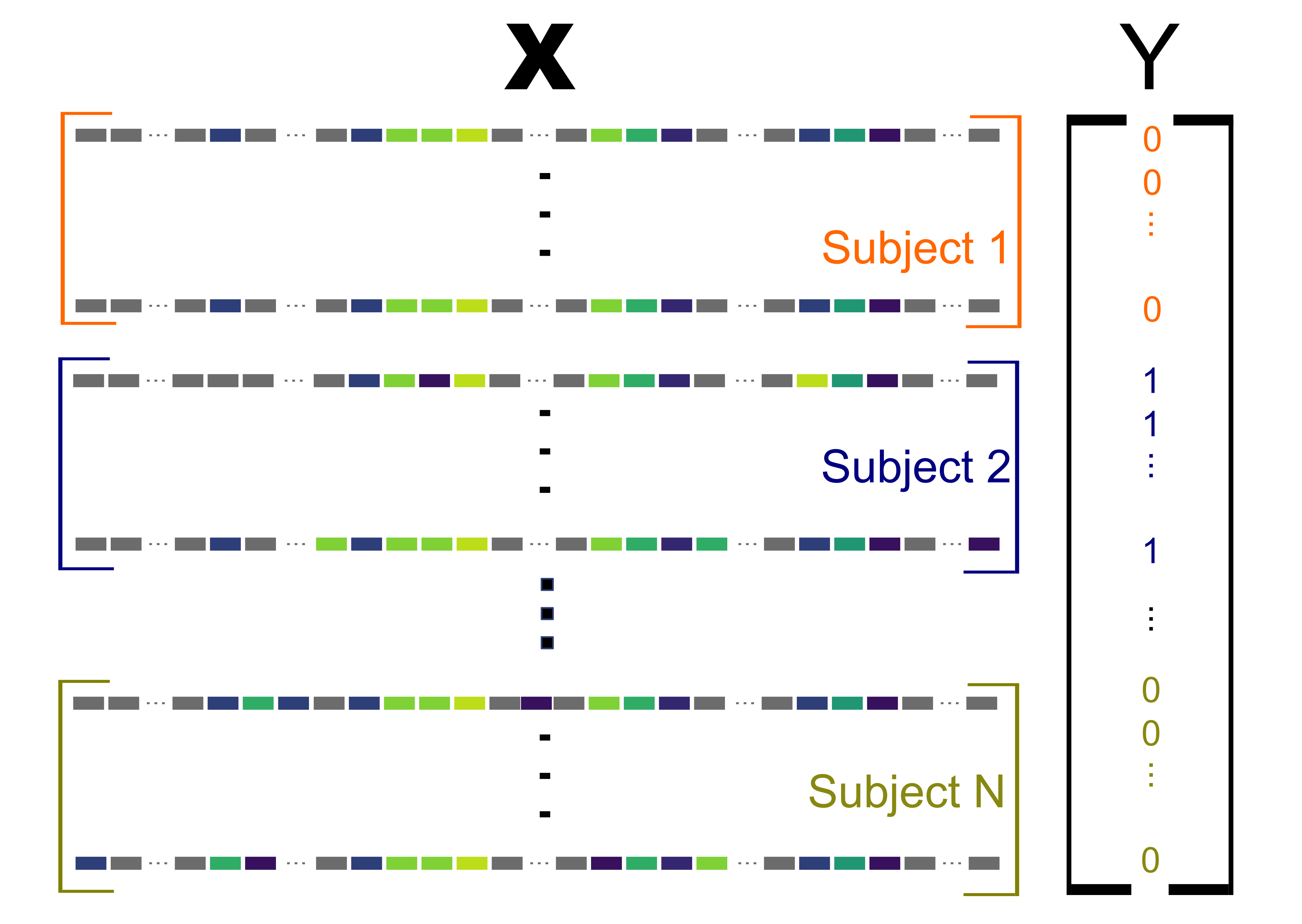
Derive predictors: repeat for all subjects
Summary
Scalar predictors and one vs. rest classification
Scalar predictors and one vs. rest classification
Aside: functional regression approach

Aside: functional regression approach

Aside: functional regression approach
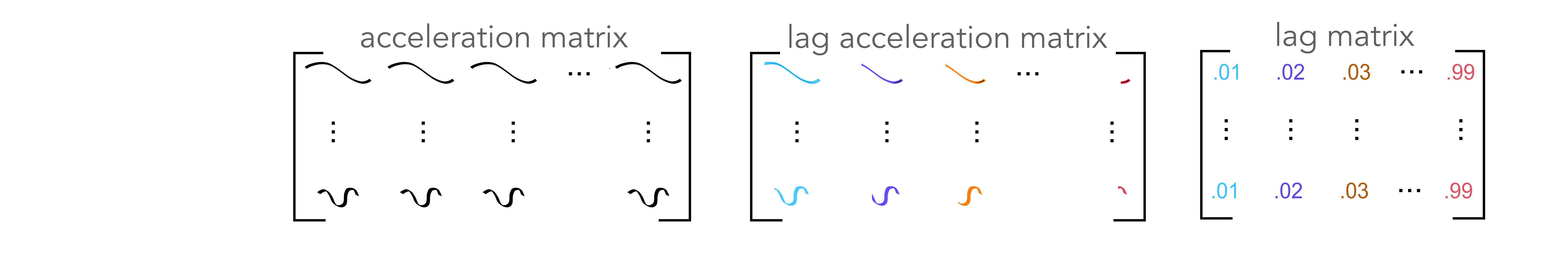
Aside: functional regression approach
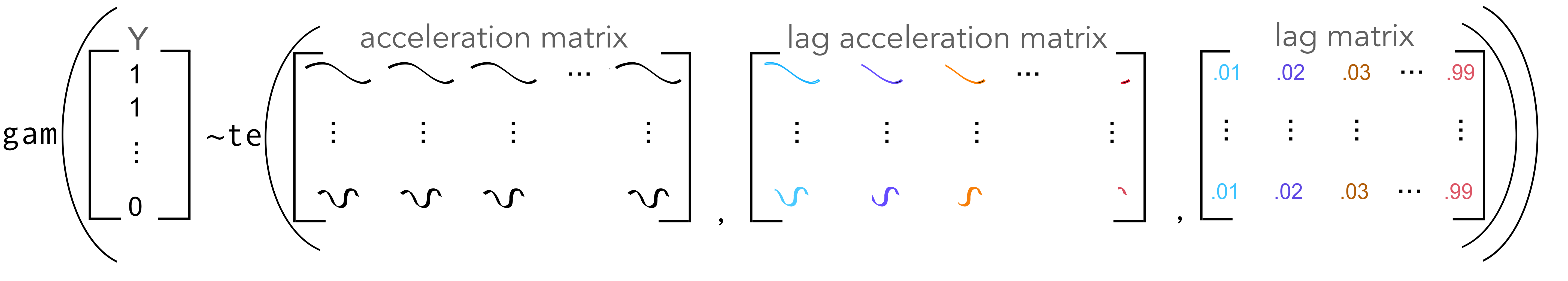
Aside: functional regression approach
\[\text{logit}(p_{ij}^{i_0}) =\beta_0^{i_0} + \int_{u=1}^S\int_{s=u}^SF_{i_0}\{ v_{ij}(s), v_{ij}(s-u), u\}dsdu \] \(u = 1, \dots, S = 100\) (number of observations per second)
\(v_{ij}(s)\) = acceleration at centisecond \(s\) for subject \(i\) in second \(j\) \(F(\cdot, \cdot, \cdot)\): trivariate smooth function
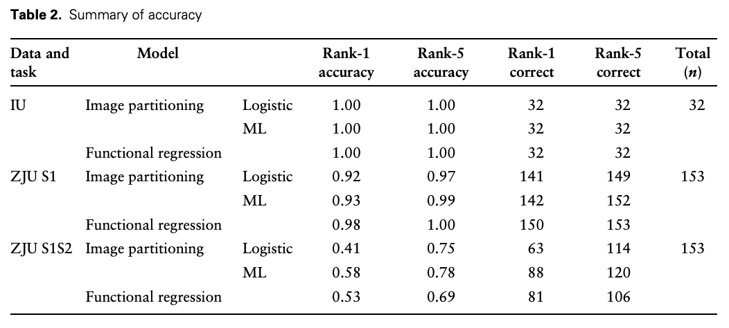
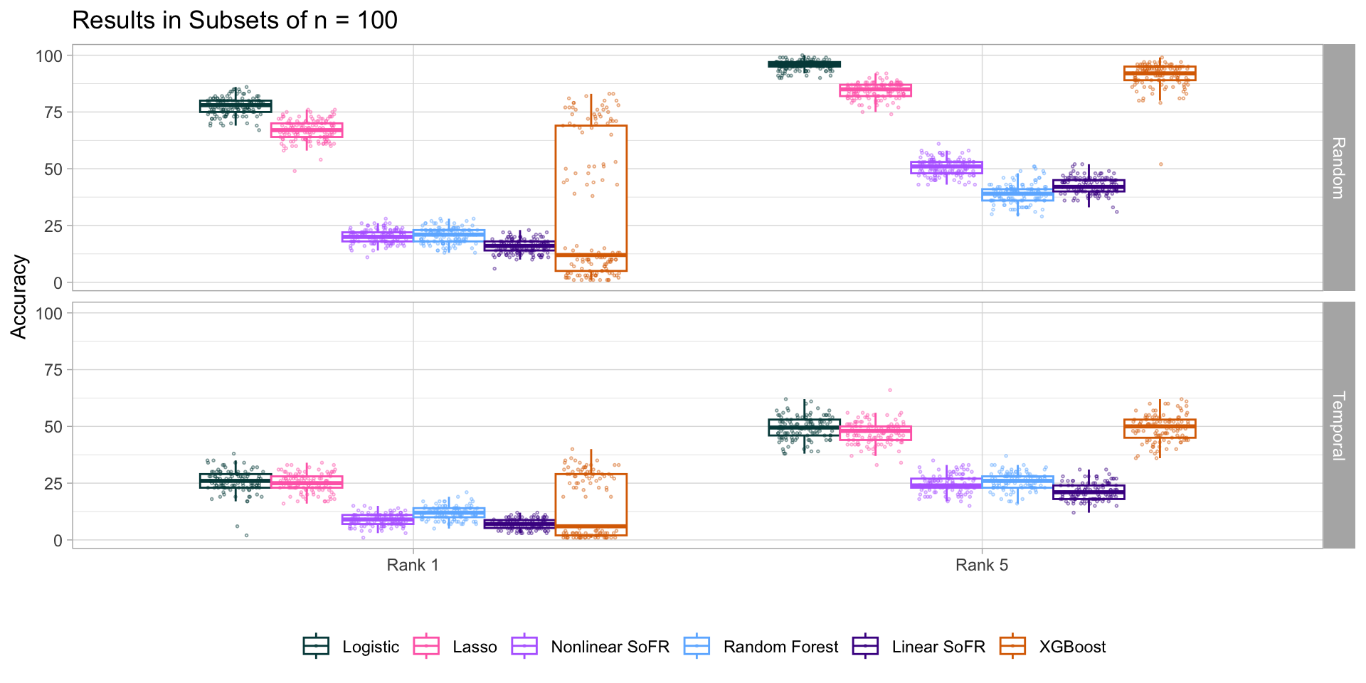
Both methods work!
Both methods work!
Both methods work!
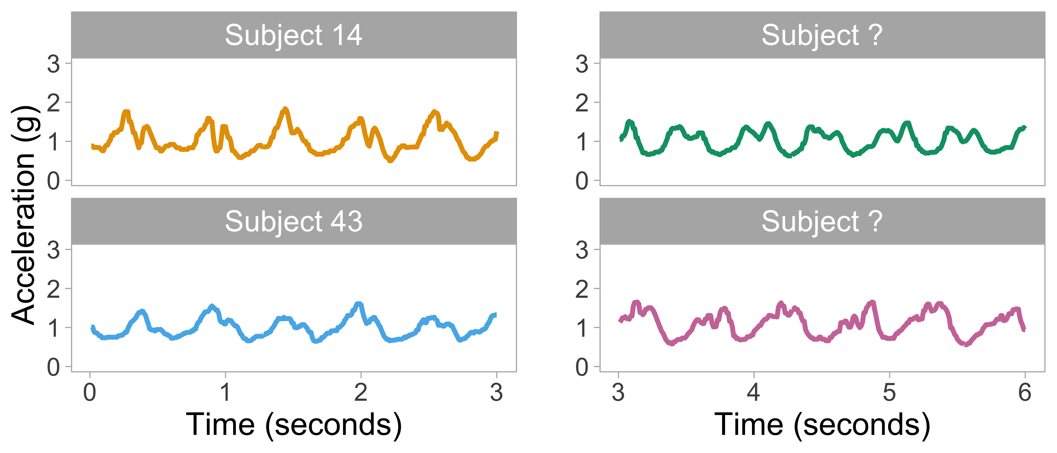
“Fingerprints” distinguish individuals
NHANES

- Biannual survey of ~5,000 Americans
- 2011-2014: wrist-worn accelerometers included in protocol
- 7 full days of free-living data from a nationally representative sample of Americans n > 15,000
- \(>10\) TB of raw data
Raw data
ADEPT templates
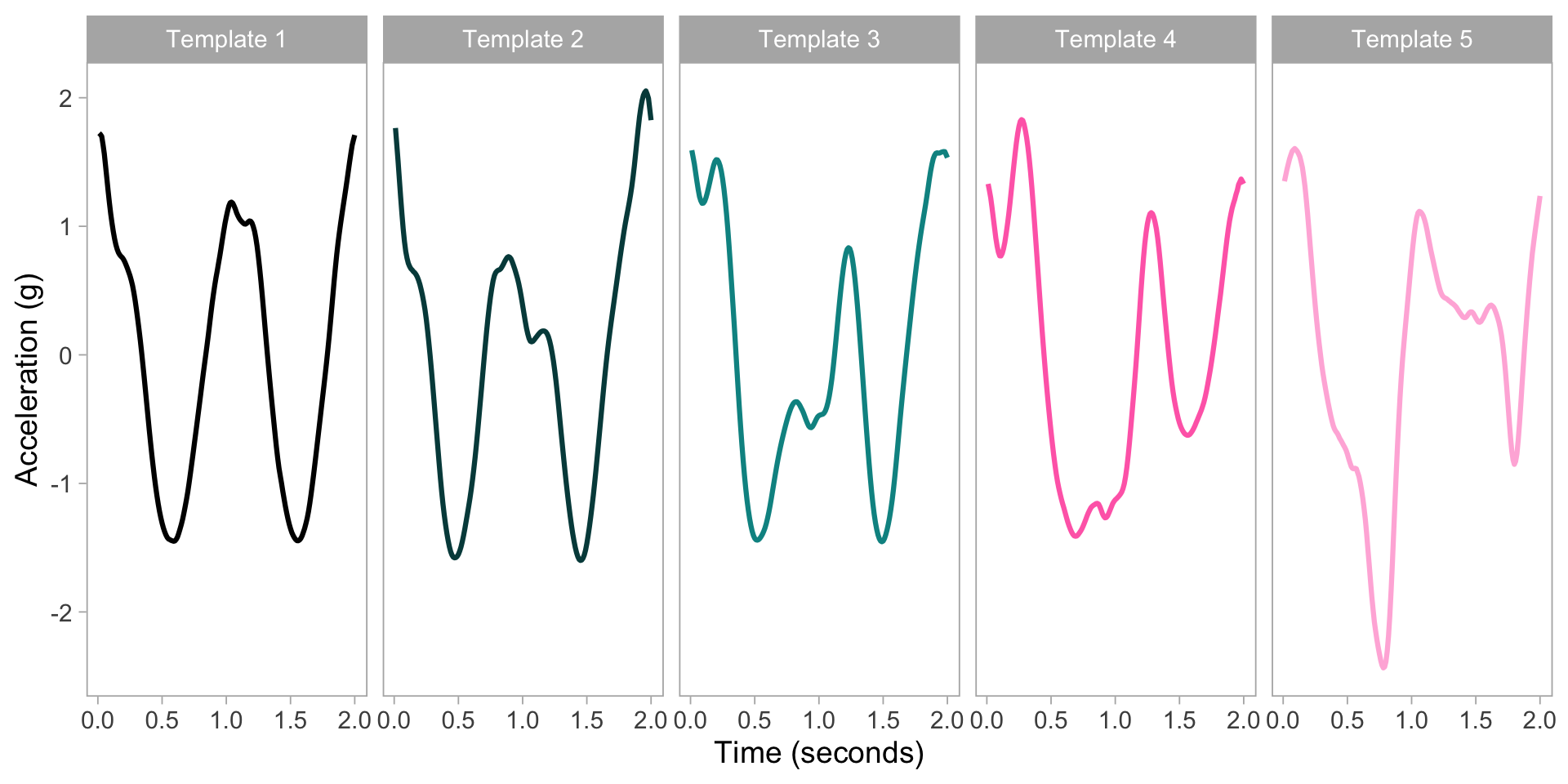
ADEPT walking identification: example
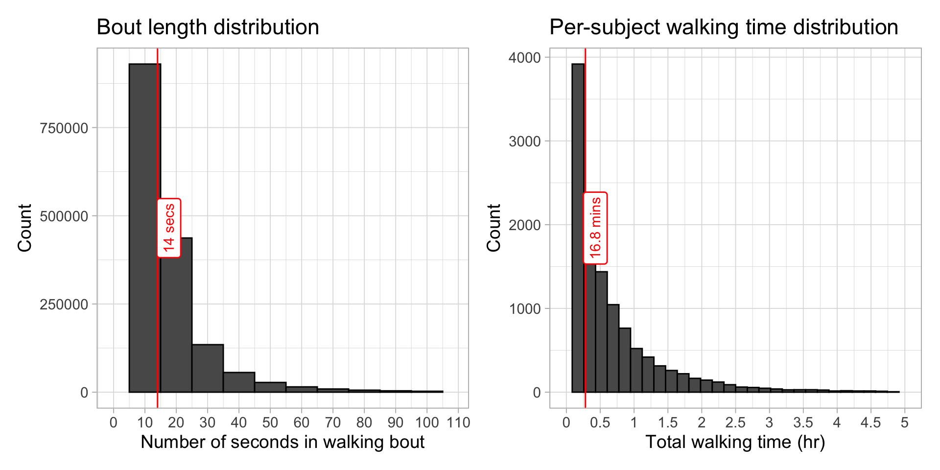
Check some results
Per-subject walking time
Define walking bout: \(\geq\) 10s where at least every other second has steps
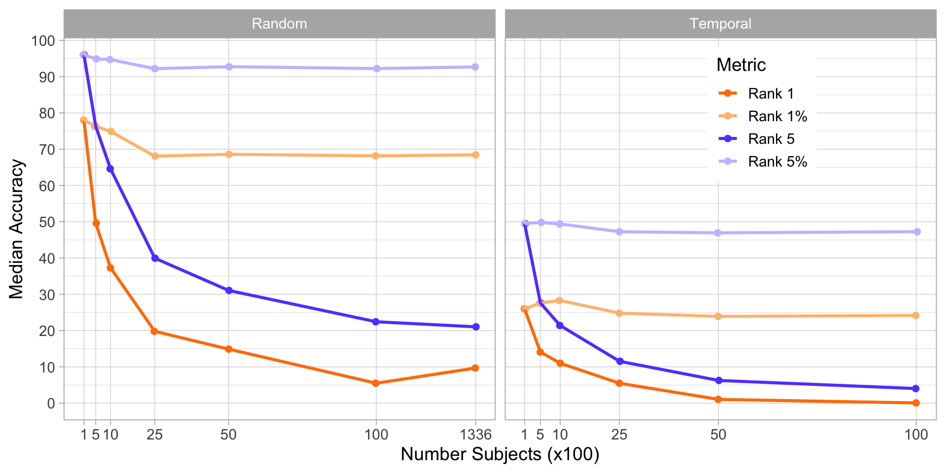
Train/test paradigms
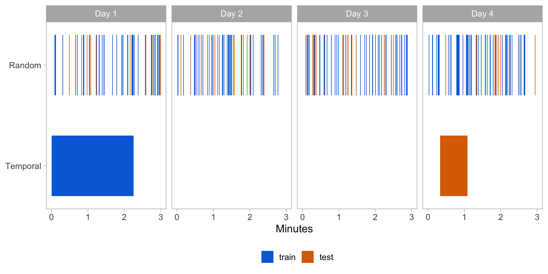
- Random: 3 minutes of walking randomly sampled from all seconds. 75% used for training, 25% used for testing. \(n = 13{,}367\) \((85\%)\)
- Temporal: 2 min 15 seconds of walking from one day used for training, 45 seconds from a later day used for testing. \(n = 10{,}770\) \((69\%)\)
Larger subsets: logistic regression
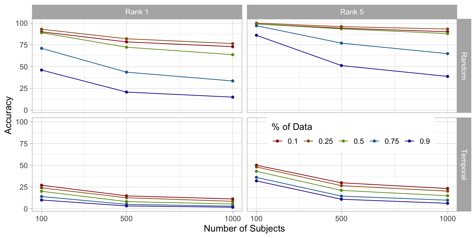
Oversampling
We can oversample the predicted subject to be a certain percent of the training data and see if this improves the model (imbalanced class)
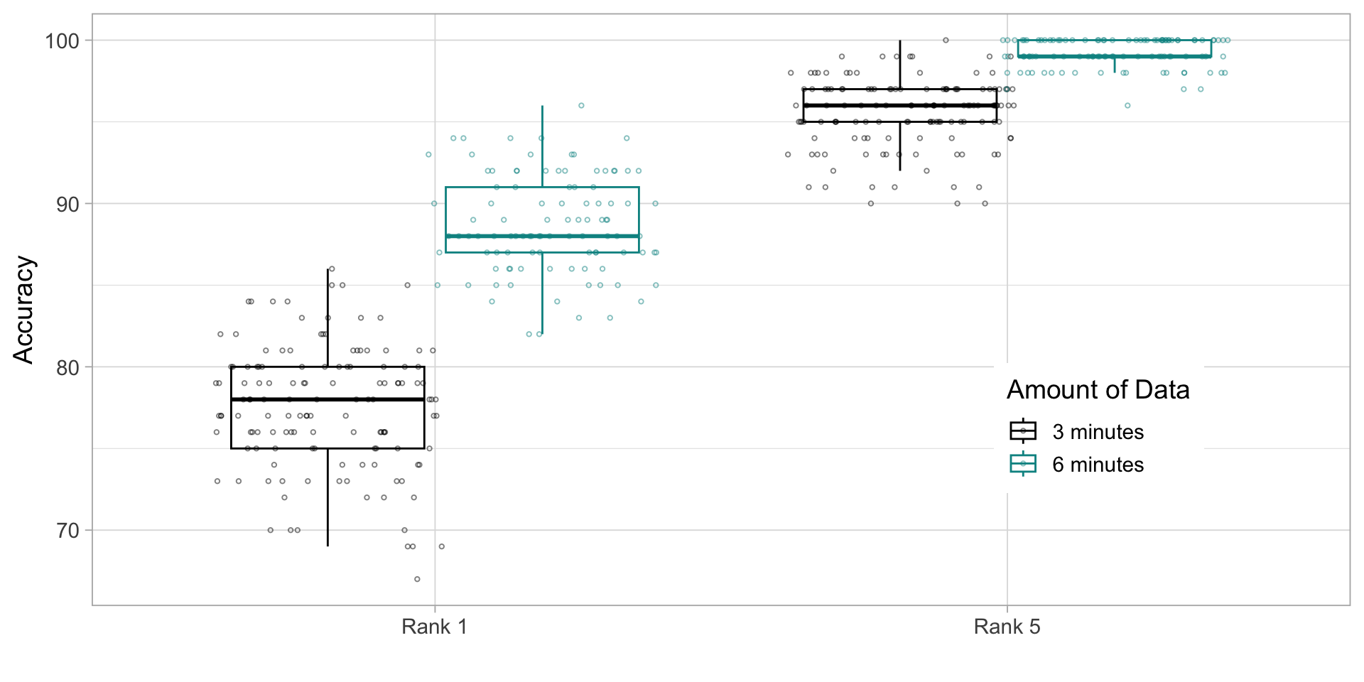
Longer training
Increase the amount of time observed for each subject to 6 minutes per person? Intuition is this should improve model performance
Fingerprints
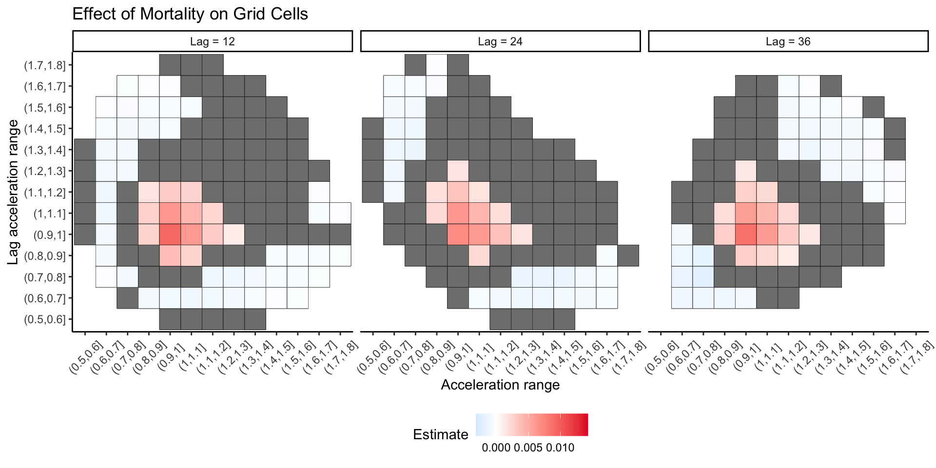
Interpret red cells as: change in 5-year mortality associated with 1% increase in time spent in cell \(c\). Next step: image on scalar regression
Thank you!
- github.com/lilykoff; lilykoff.com
- JHU collaborators: Ciprian Crainiceanu, John Muschelli, Yan Zhang, Wearable and Implantable Technology (WIT) research group
- External collaborators: Andrew Leroux (Colorado School of Public Health), Jaroslaw Harezlak (Indiana University School of Public Health)